

7. Objectives II
The objective II – tube length, apertometry
In the second part of this series of articles, it was stated that the chief role of the microscope is to present clearly-resolved detail to the eye; also the objective is the main optical element in the microscope. In the previous article on objectives (part 4), I wrote that diffraction was responsible not only for image formation but also limited the formation of the perfect image as a faithful representation of the object.
There are three types of limiting factor that affect image quality:
- optical aberrations
- image noise, and
- diffraction.
The previous article on objectives considered the various types of optical aberration found in the objective. Image noise, put simply, is merely the sum of all those factors aside of limitations due to diffraction which degrade the image as a true representation of the object. This can include the quality of the receptor or the quality of the illumination.
If we assume that we are dealing with a perfect objective, we can ignore the effects of aberrations and optical noise. Let us assume that the specimen (as lit by the lamp and condenser) is self-luminous, then the more information from the spherical wavefront that is accepted by the lens, the greater the fidelity (or faithful representation) of the image (Figure 1). In other words, the angular aperture of the lens will determine the light gathering power of the lens and, as we might expect, the larger the angular aperture the greater the fidelity of the image.
The German physicist Ernst Abbe developed the diffraction-limited theory of microscopical imaging and defined a quantitative value for the angular aperture of the lens, which he defined as numerical aperture. This is usually abbreviated as NA for short, and is given by the formula
| NA = n . sin α | (Equation 1) |
where n is the refractive index of the medium between the object and the lens, and α is half the angular aperture (see Figure 1).
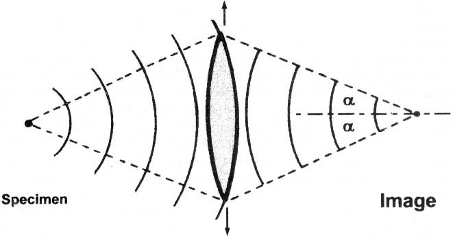
Figure 1. The larger the lens (i.e. the greater its aperture) the more information about the image is recorded.
The specimen (lit by the lamp/condenser arrangement) is considered to be formed from an infinite number of self-luminous points. We shall see the detail and features of the specimen according to how well neighbouring points are distinguished.
For two neighbouring points to be just resolvable, the distance, δ, between them is given by the formula:
| δ = 0.61 . λ/NA | (Equation 2) |
where 0.61 is a constant and λ is the wavelength of the illumination. The resolving power of the microscope, therefore, depends upon the wavelength of the illumination and the NA of the objective.
For a more detailed explanation of how this equation is derived, see Bradbury & Bracegirdle (1998) or Smith (1996a). When using white light illumination, λ may vary from 0.4 to 0.7 µm. Generally, for calculation, the mid-range value 0.55 µm for green light is assumed. For this wavelength the minimum resolvable distance is 0.336/NA. Hence determining the NA of the objective in use is very helpful for determining the performance of the microscope in resolving detail in the object. As shown in Figure 1, it is also a measure of the ‘grasp’ of the illuminating flux picked up by the objective.
In this respect, the numerical aperture of the objective is similar to the ‘f-value’ of a camera lens. The approximate relationship between f-number and NA is: given by NA ≈ 1/(2. f-number) and f-number ≈ 1/ (2.NA).
| NA | 0.03 | 0.06 | 0.1 | 0.25 | 0.5 | 1.0 | 1.4 |
| f-number | 16 | 8 | 5 | 2 | 1 | 0.5 | 0.36 |
Measurement of numerical aperture
Abbe developed the apertometer named after him, which is the most accurate method using a block of high refractive index glass (Figure 2). Light is shone evenly around the curved semi-circular rim on the front of the apertometer. It is reflected off the rear surface bevelled at 45°, by total internal reflection, and enters the objective. At the back focal plane of the objective, an image of the front rim of the apertometer can be seen. This image is magnified either by a small telescope which screws into the top of the draw-tube, or else a centring telescope (such as that used for setting-up phase contrast) may be substituted for an eyepiece. Details for making an apertometer suitable for oil-immersion objectives may be found in Haselmann (1991). With a dry objective, the term n in Equation 1 reduces to 1.0 – the refractive index of air. NA is therefore the half-angle of the maximum angular aperture of the objective, which can be measured with a swinging apertometer (Booth, 1965; Smith 1996b). A static method of measuring the NA of a dry objective, using trigonometry, is to tape the objective along a pencil line drawn on a table-top the longer this distance, the more accurate the measurement will be). At the far end, along a similarly-marked perpendicular, bring in two markers until they are just seen at the limit of the field of view. The NA can be calculated from the triangle so found.
The Cheshire apertometer (Cheshire, 1914) is simply an extension of the trigonometrical principle, using a convenient scale on the microscope stage to measure numerical aperture directly.
Optical index
The optical index (0.I.) is a term devised by E. M. Nelson, and is the ratio of the numerical aperture to the magnifying power of a lens. A multiplier of 1,000 is used to clear the expression of decimal points:
| Optical Index = [NA/Magobjective] × 1,000 | (Equation 3) |
The optical index is closely related to the ‘f-number’ of the camera, but magnifying power is used instead of focal length which is a small distance in the microscope, and difficult to measure with sufficient accuracy for calculation. Nelson intended the Optical Index to be a convenient way of comparing objectives of different numerical aperture. The higher the Optical Index of an objective, the better is its light-gathering power and also its ability to convey detail into the image.
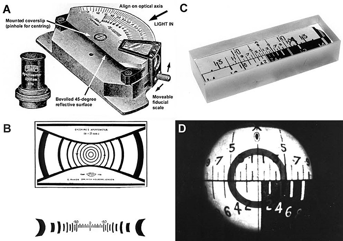
Figure 2. A drawing of various types of apertometer. (A) the Abbe Apertometer, together with the telescope supplied to view the back focal plane of he objective. (B) the Cheshire apertometer, a dry form of apertometer, based on trigonometry. (C) the Beck glass block apertometer; it can be used dry or with oil. (D) the Beck apertometer in use. The phase plate of the objective can be seen in the back focal plane superimposed over the apertometer scale; the scale is curved by the objective, making it difficult to read at the periphery, which is why Cheshire printed his apertometer with a curved scale.
From equation (2), above, the minimum resolvable distance is approximately 0.34/NA. Human eyes vary in visual acuity, but it is generally accepted that the smallest distance between two points resolvable by the naked eye is 90 µm. Therefore, the minimum overall magnification necessary to resolve detail in a microscopical specimen (µm units cancel out) is:
| 90/[0.34/NA] = 90.[2.94NA] ≈ 260.NA | (Equation 4) |
If the microscope is used with a ×10 eyepiece, then an objective must have an optical index of at least 26 to be theoretically perfect. A modern achromatic ×10 objective with a NA of 0.30 will have an optical index of 30. An oil-immersion apochromat ×40 of NA 1.4 will have an O.I. of 35, while an oil-immersion apochromat ×63 of NA 1.4 will have an O.I. of 22. An achromat of ×100 magnification, with NA of 1.3 will have an O.I. of 13. Since aperture is more costly and difficult to incorporate into an objective than magnifying power, the O.I. also provides a comparison of monetary value and quality between objectives. It is beyond the scope of this article, but the optical index also provides a sound means of matching video and CCD cameras to the objectives used for imaging.
The magnifying power of an objective, which may vary by a few percent from the inscription on the barrel, can be precisely determined by directly measuring the image of a stage micrometer at the primary image plane. It may also be determined by dividing the overall magnification of the microscope by the magnifying power of the eyepiece or, where applicable, the product of the eyepiece and any intermediate magnification changers. Unfortunately, space precludes a detailed description of the means of determining accurately the magnifying power of the objective and eyepiece and the measurement of focal length. Interested readers are referred to Dade (1955).
Tube lengths in the microscope
Every objective lens is computed to form an image at the primary image plane (PIP), which is then magnified by the eyepiece. To ensure that the image is sharp, and that the diaphragm at the front focal plane of the eyepiece is precisely located where the objective will form the primary image, there is a standard distance, the mechanical tube length, MTL, which is the distance (in millimetres) from the objective thread collar to the top of the tube into which the eyepiece slips (Figure 3). This used to be 250 mm – the ‘old English’ measurement of 10 inches. Towards the close of the nineteenth century, the ‘continental’ standard of 160 mm began to be widely adopted, although the firm of Leitz adopted 170 mm until recently. The mechanical tube length for which a particular objective has been computed is usually engraved on the objective barrel. Generally, the eyepiece is constructed so that its front focal plane, designed to be coincident with the PIP, is 10 mm inside the microscope body-tube from the top.
The optical tube length, OTL, is different from the mechanical tube length. The OTL is the distance between the back focal plane of the objective and the primary image plane (Figure 3). The OTL is not a standardised length because objectives of different magnifying power have different focal lengths. The higher the magnification of the objective, the shorter the focal length. For convenience manufacturers compute their objectives to be parfocal. This means that they will all focus on the specimen (within small limits) whichever objective is swung into use on the nosepiece. For this reason, the higher the magnification of the objective, the deeper the back focal plane of the objective (fobj in Figure 3) is located within the lens elements, and the longer the optical tube length. Only very simple achromats of low power will have a back focal plane located outside the barrel of the objective. For a method of how to measure the optical tube length for a particular objective, see Dade (1955).
Within the body-tube the rays of image-forming light are not parallel, but converge to form the primary image. It is therefore a complex task for the optical designer to elongate the tube lengths in order to insert extra equipment, such as incident-light illuminators or contrast-enhancing equipment, in the microscope body-tube. Most firms have now turned to manufacturing ‘infinity-corrected’ optics, where the tube length is theoretically infinite. The specimen is viewed at the front focal plane of the objective, so that the image-forming rays emanating from the objective are parallel. They are then brought to a focus at the front focal plane of the eyepiece by a single lens element – the ‘tube lens’. This then allows the designer extra space between the objective and eyepiece in which to put extra equipment without having to incorporate many extra lens elements to maintain the primary image at its proper location. The infinity-corrected system is not illustrated, since most members will still own so-called ‘finite tube-length’ or ‘classical tube-length’ instruments. Infinity corrected objectives are marked ∞ on the barrel, and cannot be exchanged for use with finite tube length objectives.
Use of a draw tube, or objective with a correction collar
As the numerical aperture of the objective increases, it is more difficult to correct for spherical and chromatic aberration. Using compensating eyepieces to correct for lateral chromatic aberration was discussed in the previous article on objectives. Here I wish to discuss the various options available for correcting residual spherical aberration in the image.
Each objective is corrected for spherical aberration at its defined optical tube length, so that a perfect image is formed at the primary image plane, as stated earlier. If the specimen is effectively ‘shifted’ from the point of focus of the objective, then the primary image will suffer from spherical aberration. This ‘shifting’ will result from using a coverslip that is either too thick or thin from the standard (usually 170 ± 5 µm) for which the objective is designed. Too much mounting medium, or a change in its refractive index, will also mimic the effect of changing the thickness of the coverslip. The coverslip thickness for which the objective is computed is engraved alongside the mechanical tube length, e.g. 160/0.17. Where the numerical aperture is sufficiently low (usually less than NA 0.5) for the coverslip thickness to be immaterial, the 0.17 is replaced by a dash, thus: 160/–. For critical work, the specimen should be deposited directly onto the lower face of a measured coverslip of exactly 0.17 mm, and the mounting medium (which can now be of any convenient depth) added between the specimen and the slide. In a monocular microscope, such as that shown in the diagram below (Figure 3), the remedy is simple.
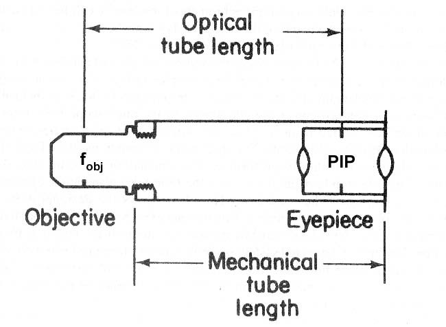
Figure 3. A diagram illustrating mechanical and optical tube lengths.
The eyepiece is housed in a separate drawtube which slides within the body tube of the microscope. The PIP is then slid into its correct position to maintain the correct optical tube length by alteration of the mechanical tube length. Space precludes a description of the exact procedure; for details see the article by Dodge (1998, Bulletin No. 32, pp. 29–33), where the first article on objectives was published.
An objective with an NA of 0.45 has only half the resolving power of one with NA 0.90, regardless of magnification; tube length correction is more critical with dry objectives of high numerical aperture, in order to minimize spherical aberration. When spherical aberration is caused by working conditions not as the manufacturer intended, the effect will be seen upon points seen as out-of-focus images slightly above or below focus. With no spherical aberration an image point should expand equally either side of focus. Where unequal images are present either side of focus, then spherical aberration is present to some degree. If a hazy disc with a bright spot in the centre is seen on focusing upwards and a sharply-defined annular ring seen on focusing downwards, the coverglass is too thin, the system is spherically under-corrected and the tube length should be increased. The rule of thumb is ‘ring down tube up’. Conversely, if a hazy disc of light with a bright central spot is seen on focusing downwards, and a bright ring on focusing upwards, the coverglass is too thick, the system is over-corrected and the tube length should be decreased. Do not use an alteration of the tube length with the draw-tube to give a slight change in magnifying power, since this obviously will introduce unwanted spherical aberration.
It is not possible to mount a drawtube on a microscope with a binocular head. In this case the alteration for spherical aberration is made within the objective itself. Those objectives that are particularly sensitive to spherical aberration are those dry lenses of high numerical aperture (usually NA 0.95), colloquially termed ‘high-dry’ objectives. They are fitted with a rotating correction collar which in so doing acts upon the rear lens elements to alter the optical tube length as appropriate. Using a correction collar is tricky and requires practice. Focus the image as near perfectly as possible, turn the collar and refocus. Consider whether the image is better or worse and turn the collar as appropriate until the optimum image is secured. In the next article stereomicroscopy will be discussed.
References
Booth, A. D. (1965.) The measurement of numerical aperture. Jour. Quekett Microscopical Club Series 4, 7:95–99.
Bradbury, S. & Bracegirdle, B. (1998). Introduction to Light Microscopy Bios Scientific Publishers, Oxford. ISBN 1-859961-21-5
Cheshire, F. J. (1914). Two simple apertometers for dry lenses. Jour. Quekett Microscopical Club Series 2, 12:283–286.
Dade, H. A. (1955). Simple microscopical determinations. Jour. Quekett Microscopical Club Series 4, 4:185–195.
Dodge, V. (1998). Tube length adjustment, how important is it? Bulletin of the Quekett Microscopical Club No. 32: 29–33.
Haselmann, H. (1991). A mini-apertometer. Proc. Royal Microscopical Soc. 26/4: 217–221.
Smith, M. (1996a). The measurement of numerical aperture (part 1) Balsam Post 30:24–27.
Smith, M. (1996b). The measurement of numerical aperture (part 2) Balsam Post 31:29–31.
© Jeremy Sanderson, Oxford, 2010